Pairs Trading & Statistical Arbitrage: Profiting From the Spread Between Two Correlated Stocks

A Different Question: Not One Stock, But the Relationship Between Two

Every mean-reversion strategy covered so far in this course (Lessons 3 and 10) asks whether a single stock has strayed from its own average — a moving average, a Bollinger Band, a VWAP. Pairs trading asks a different question entirely: has the price relationship between two stocks that normally move together strayed from its own historical norm?

Take two chipmakers exposed to the same semiconductor cycle. They tend to drift in the same direction most of the time, because they share the same macro exposure. But if one suddenly rallies hard for a few sessions while the other sits flat, you're left with a judgment call: is that gap a genuine change in each company's fundamentals, or just a temporary imbalance in order flow? Pairs trading is built on betting the latter — that a temporary dislocation between two historically linked prices tends to narrow again.

This is usually introduced as the original, simplest form of a broader category called statistical arbitrage (stat arb). Large quant funds — Renaissance Technologies, D.E. Shaw, and Two Sigma are commonly cited examples — are known to run heavily engineered versions of this same core idea. One thing worth being upfront about: it's widely acknowledged in the industry that the easy, simple pairs-trading edges retail traders could once capture in the 1990s and early 2000s have eroded substantially now that algorithmic trading accounts for the majority of equity volume. That doesn't make the underlying logic useless, though — it's still a genuinely useful framework for understanding how to construct a position that's largely indifferent to overall market direction.

The Core Mechanic: A Market-Neutral Position Built From Long/Short

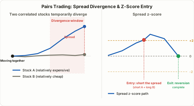
The structure is straightforward. Given two stocks A and B that historically move together:

• When the spread between them widens abnormally: short the one that's become relatively expensive, and buy the one that's become relatively cheap.
• When the spread narrows back to its normal range: close both legs simultaneously and take the profit.

The key point is that it doesn't matter whether either stock goes up or down in absolute terms. If you're long one chipmaker and short the other, it doesn't matter whether both rally because the whole sector re-rates, or both fall because the broader market sells off — your P&L is driven purely by the relative gap between them. This property is called market neutrality, and it's the biggest structural difference from every directional strategy covered earlier in this course: a market-neutral pair can profit even while the index goes sideways or down, as long as the spread widens and then narrows. That said, this assumes the two legs' gains and losses genuinely offset each other in practice — they rarely do so perfectly, which is a caveat we'll return to below.

Correlation Alone Isn't Enough: Why Cointegration Matters

The first instinct when hunting for a pair is to check the correlation coefficient between two price series. But picking pairs on correlation alone is a common trap, because correlation only tells you whether two prices have tended to move in the same direction — it says nothing about whether the relationship stays confined to a stable range over time. Two stocks can drift up together for a few months by coincidence, with no real structural link between them; correlation reads high, but nothing guarantees the spread narrows again — it can just as easily widen indefinitely in one direction.

The property quant traders actually care more about is cointegration. In plain terms:

Concept	What it measures	Limitation
Correlation	How closely two price series move in the same direction	Can read high purely by short-term coincidence
Cointegration	Whether the difference (spread) between the two prices itself has a tendency to revert to a stable mean	Harder to test rigorously, and a historical relationship holding is no guarantee it holds going forward

In practice, you don't necessarily need a formal cointegration test (like an Engle-Granger test) to get some of this benefit. Choosing pairs from the same industry, similar business models, or overlapping supply chains — two chipmakers, Coca-Cola and Pepsi, two telecom carriers in the same market — gives you a fundamental reason the two prices should track each other over the long run. Pairing two unrelated stocks purely because a recent correlation reading happens to be high is one of the most commonly cited mistakes in this strategy.

Calculating the Spread and the Z-Score

To turn pairs trading into a rule-based system, you need a number that expresses "how far has the spread strayed from normal." The standard sequence is:

Step 1 — Define the spread. The simplest version uses the price ratio (A ÷ B) directly as the spread. A more rigorous version regresses A on B (an OLS regression) to derive a hedge ratio (β), then defines the spread as A − β×B. Using a hedge ratio also tells you directly how many shares of B to trade against one share of A to keep both legs dollar-neutral.

Step 2 — Compute a rolling mean and standard deviation. Using the trailing N sessions (a 20–60 day lookback is commonly referenced — this is a widely used convention, not a validated optimum), calculate the moving average and standard deviation of the spread.

Step 3 — Compute the z-score.

z-score = (today's spread − rolling mean) ÷ rolling standard deviation

The z-score tells you how many standard deviations today's spread sits from its recent average. A z-score of +2 means the spread has widened to a level that's statistically unusual relative to its recent history; −2 means the opposite — it has narrowed unusually far.

Entry, Exit, and Stop-Loss Rules

Once you have a z-score, the trading rules become fairly mechanical. The thresholds below are commonly referenced conventions from quant trading education and community practice — treat them as a starting point, not a validated fixed rule.

Situation	Z-score condition (convention)	Action
Spread abnormally wide	z ≥ +2	Bet on spread narrowing: short A, buy B
Spread abnormally narrow	z ≤ −2	Bet on spread widening: buy A, short B
Mean reversion complete	z returns near 0	Close both legs simultaneously, take profit
Relationship possibly broken	z ≥ +3 to +4 (or a fixed loss limit is hit)	Stop-loss: assume the spread won't revert, exit both legs

That last row matters most. The fact that a z-score has no hard ceiling — it can keep widening indefinitely — is this strategy's single biggest risk. Holding a spread trade without a stop because "it's stretched this far, it has to come back" is the same underlying mistake mean-reversion strategies elsewhere in this course warn against — catching a falling knife. In pairs trading, this failure mode is often described as "picking up nickels in front of a steamroller": reversion is a statistical tendency the spread has shown historically, not a law that guarantees it happens again.

A Worked Numeric Example

Assume two hypothetical chipmakers, A (large-cap) and B (mid-cap), that have historically moved together. Over the trailing 30 sessions, the price ratio (A ÷ B) has averaged 2.40 with a standard deviation of 0.05.

Today, A trades at $54.00 and B at $21.75, giving a ratio of 54.00 ÷ 21.75 ≈ 2.483.

z-score = (2.483 − 2.40) ÷ 0.05 = 1.66

That's still short of the conventional ±2 entry threshold. Suppose the next session A climbs further to $55.20 while B slips slightly to $21.63, pushing the ratio to 2.552:

z-score = (2.552 − 2.40) ÷ 0.05 = 3.04

At this point the spread has blown through the conventional entry threshold (+2) and is approaching the stop-loss zone (+3 to +4). A conservative trader would rather have entered earlier — right as the z-score first crossed +2, shorting A and buying B — and then closed both legs once the ratio drifted back toward the 2.40 mean, rather than initiating a fresh position this far into an already-extended move. If the ratio instead kept climbing past 3.0, that would be a signal the underlying fundamental relationship between the two companies may have genuinely shifted, and the stop-loss rule should trigger a full exit.

Why Market Neutrality Is Both the Edge and the Cost

The biggest appeal of pairs trading is its low correlation to directional strategies. Even during a sharp index selloff, a well-chosen pair whose spread stays within its normal range can hold up largely independent of what the broader market is doing. Layered into a portfolio otherwise built from directional strategies — in the spirit of Lesson 6's Risk-Reward & Money Management — this can meaningfully reduce overall account volatility through diversification.

That structure isn't free, though.

• Trading costs are effectively doubled. A single round-trip trade means buying and selling two separate stocks — four total executions — so commissions and slippage stack up faster than with a single-stock strategy.
• The short leg carries borrow costs and constraints. Shorting a stock requires shares to be available to borrow, often at a fee, with terms that can force an early close — and for some names, borrow may not be available at all.
• A perfect hedge is closer to theory than reality. Even a carefully estimated hedge ratio (β) drifts over time as each stock's sensitivity changes, so in practice a pairs trade is better described as "much less sensitive to market direction" than "100% market neutral."

Limitations and Caveats

• Structural break risk. The largest losses in pairs trading almost always come from the core assumption — that the spread will revert — simply failing. A merger, an earnings shock, or a regulatory event hitting only one of the two companies can permanently sever a relationship that held for years. A predefined stop-loss is not optional here.
• Pairs need periodic re-validation. A relationship that worked in the past isn't guaranteed to keep working. Industry shifts, business diversification, or index inclusion/exclusion changes can quietly erode a correlation over time, so re-checking whether a pair's relationship still holds on something like a quarterly basis is a reasonable habit.
• The easy edge is widely believed to have shrunk. As noted above, simple pairs trading is a well-known technique that institutional algorithms compete over heavily. For an individual trader, it's more realistic to treat this as a diversification and risk-management tool within a broader portfolio than as a reliably repeatable source of alpha on its own.
• Vulnerable to backtest overfitting. Parameters like the entry threshold (z = 2) and the lookback window (20–60 days) are easy to over-tune against historical data in a way that doesn't hold up going forward. Keeping parameters at simple, round-number values reduces (though doesn't eliminate) this risk.

Summary

• Pairs trading looks at the relative price gap (the spread) between two historically correlated stocks, rather than a single stock's deviation from its own average.
• When the spread widens abnormally, short the relatively expensive stock and buy the relatively cheap one to build a market-neutral position; close both legs together once the spread reverts toward its mean.
• Cointegration — whether the spread itself tends to revert — matters more than raw correlation; in practice, choosing pairs from the same industry or business model is a reasonable proxy for this.
• Normalizing the spread into a z-score and using roughly ±2 as an entry trigger, 0 as an exit trigger, and ±3 to +4 as a stop-loss are commonly referenced conventions, not validated fixed rules.
• Market neutrality lowers correlation to overall market direction, but comes at the cost of doubled trading costs, short-borrow constraints, and an imperfect hedge.
• The biggest risk is a structural break — the relationship simply failing to revert — so always trade this with a predefined stop-loss and the position-sizing discipline from Lesson 6.